Vector Search

Since version 4.0, Apache Doris natively supports ANN (Approximate Nearest Neighbor) vector search. Built on Faiss with HNSW and IVF indexes, it delivers millisecond-level TopN and range retrieval over billions of vectors.

Applicable Scenarios

Vector search is the core capability behind RAG (Retrieval-Augmented Generation) and multimodal retrieval. Typical applications include:

• RAG retrieval: Retrieve the Top-K text snippets most relevant to a user query from a large knowledge base, and use them as the basis for LLM generation. This mitigates hallucination and knowledge-staleness issues.
• Multimodal retrieval: Encode images, audio, video, and other data into vectors for semantic similarity queries. For example, in medical Q&A, retrieve case records and literature to assist diagnostic suggestions.
• Recommendation systems: Use range search to retrieve "similar but not identical" candidate content, improving recommendation diversity.
• Anomaly detection: Locate data points that deviate from normal patterns.

The essence of vector retrieval is: encode the query and documents into semantic vectors using the same scheme, then find the K vectors most similar to the query from a large vector collection.

Quick Navigation

Scenario	Section
Learn how to create a vector index	Approximate Nearest Neighbor Search
Implement Cosine similarity retrieval	Using Cosine Similarity
Filter by distance threshold	Approximate Range Search
Combine TopN with range conditions	Compound Search
Filter by other columns before ANN retrieval	ANN Search with Filters
Tune query behavior parameters	Query Parameters
Save memory and reduce index size	Vector Quantization
Improve QPS and reduce latency	Performance Tuning
Use the Python SDK	Python SDK
Learn about usage limitations	Usage Limitations

---

Approximate Nearest Neighbor Search

Doris does not introduce a new data type. Vectors are stored as fixed-length Array<Float>, and a Faiss-based ANN index type is provided for distance retrieval.

Table Creation Example

Take the common SIFT dataset as an example:

CREATE TABLE sift_1M (
  id int NOT NULL,
  embedding array<float>  NOT NULL  COMMENT "",
  INDEX ann_index (embedding) USING ANN PROPERTIES(
      "index_type"="hnsw",
      "metric_type"="l2_distance",
      "dim"="128",
      "quantizer"="flat"
  )
) ENGINE=OLAP
DUPLICATE KEY(id) COMMENT "OLAP"
DISTRIBUTED BY HASH(id) BUCKETS 1
PROPERTIES (
  "replication_num" = "1"
);

Meaning of each core parameter:

• index_type: The index algorithm. Options are hnsw (Hierarchical Navigable Small World), ivf (Inverted File index), or ivf_on_disk (an IVF variant whose inverted lists are written to disk and served through a cache).
• metric_type: The distance metric. l2_distance means using L2 distance as the distance function.
• dim: The vector dimension. 128 means each vector in this column has length 128.
• quantizer: The encoding scheme. flat means each dimension is stored as the original float32 value.

Full Index Parameters

Parameter	Required	Supported / Optional Values	Default	Description
index_type	Yes	hnsw, ivf, ivf_on_disk	(none)	Specifies the ANN index algorithm. Currently HNSW, in-memory IVF, and IVF On-Disk are supported.
metric_type	Yes	l2_distance, inner_product	(none)	Specifies the vector similarity / distance metric. l2_distance is Euclidean distance. inner_product can be used for cosine similarity scenarios, but the vectors must be normalized first.
dim	Yes	Positive integer (> 0)	(none)	Specifies the vector dimension. All vectors loaded later must have the same dimension, otherwise an error is reported.
nlist	No	Positive integer	1024	Number of inverted buckets in IVF. Takes effect when index_type=ivf or ivf_on_disk. A larger value usually offers a better recall/speed trade-off but increases build cost.
max_degree	No	Positive integer	32	Maximum number of neighbors per node in the HNSW graph (M). Affects index memory usage and search performance.
ef_construction	No	Positive integer	40	Size of the candidate queue during HNSW construction (efConstruction). A larger value yields a higher-quality graph but slower build.
quantizer	No	flat, sq8, sq4, pq	flat	Vector encoding / quantization scheme. flat: original storage. sq8 / sq4: scalar quantization (8 / 4 bit). pq: product quantization.
pq_m	Required when quantizer=pq	Positive integer	(none)	The number of sub-vectors the original high-dimensional vector is split into. dim must be divisible by pq_m.
pq_nbits	Required when quantizer=pq	Positive integer	(none)	The number of bits used to quantize each sub-vector, which determines the codebook size of the subspace (k = 2 ^ pq_nbits). In Faiss this is generally required to be no greater than 24.

Data Loading

Load the SIFT dataset through the S3 TVF:

INSERT INTO sift_1M
SELECT *
FROM S3(
  "uri" = "https://selectdb-customers-tools-bj.oss-cn-beijing.aliyuncs.com/sift_database.tsv",
  "format" = "csv");

select count(*) from sift_1M
--------------

+----------+
| count(*) |
+----------+
|  1000000 |
+----------+

Query Example

Calling l2_distance_approximate / inner_product_approximate triggers the ANN index path.

Calling rules:

• The function name must exactly match the index metric_type:
  • metric_type=l2_distance → use l2_distance_approximate
  • metric_type=inner_product → use inner_product_approximate
• Sort order:
  • L2 distance uses ascending order (ORDER BY dist ASC, smaller is closer).
  • Inner product uses descending order (ORDER BY dist DESC, larger is closer).

SELECT id,
       l2_distance_approximate(
        embedding,
        [0,11,77,24,3,0,0,0,28,70,125,8,0,0,0,0,44,35,50,45,9,0,0,0,4,0,4,56,18,0,3,9,16,17,59,10,10,8,57,57,100,105,125,41,1,0,6,92,8,14,73,125,29,7,0,5,0,0,8,124,66,6,3,1,63,5,0,1,49,32,17,35,125,21,0,3,2,12,6,109,21,0,0,35,74,125,14,23,0,0,6,50,25,70,64,7,59,18,7,16,22,5,0,1,125,23,1,0,7,30,14,32,4,0,2,2,59,125,19,4,0,0,2,1,6,53,33,2]
       ) AS distance
FROM sift_1M
ORDER BY distance
LIMIT 10;
--------------

+--------+----------+
| id     | distance |
+--------+----------+
| 178811 | 210.1595 |
| 177646 | 217.0161 |
| 181997 | 218.5406 |
| 181605 | 219.2989 |
| 821938 | 221.7228 |
| 807785 | 226.7135 |
| 716433 | 227.3148 |
| 358802 | 230.7314 |
| 803100 | 230.9112 |
| 866737 | 231.6441 |
+--------+----------+
10 rows in set (0.02 sec)

To compare with exact results, use l2_distance / inner_product (without the _approximate suffix). In this example, the exact search takes about 290 ms; with the ANN index, query latency drops from about 290 ms to about 20 ms.

10 rows in set (0.29 sec)

Execution Mechanism

The ANN index is built at the segment granularity. In a distributed table:

1. Each segment returns its local TopN results.
2. The TopN operator merges results across tablets and segments to produce the global TopN.

---

Using Cosine Similarity

The Doris ANN index metric_type currently supports only l2_distance and inner_product, and does not directly support cosine. When the business metric is cosine similarity, you can convert it equivalently to inner product through normalization.

Steps

1. Before writing: L2-normalize the vectors (normalize to unit length).
2. When creating the index: Use metric_type="inner_product".
3. When querying: Use inner_product_approximate(...), sorted by ORDER BY ... DESC.

Example:

CREATE INDEX idx_emb_cosine ON your_table (embedding) USING ANN PROPERTIES (
  "index_type"="hnsw",
  "metric_type"="inner_product",
  "dim"="768"
);

Equivalence Rationale

• Cosine similarity formula: cos(x, y) = (x · y) / (||x|| ||y||)
• When the vectors are L2-normalized (||x|| = ||y|| = 1): cos(x, y) = x · y

Therefore, in unit-vector space, maximizing cosine similarity is equivalent to maximizing inner product. Without normalization, inner product and cosine are no longer equivalent.

---

Approximate Range Search

Beyond TopN nearest-neighbor search, vector retrieval has another common query type: range search based on a distance threshold. Such a query does not return a fixed number of rows. Instead, it finds all data points whose distance to the target vector satisfies the condition.

Typical applications:

• In recommendation systems, retrieve content that is "close but not identical" to increase diversity.
• In anomaly detection, locate data points that deviate from normal patterns.

Example: count rows whose L2 distance to the target vector is greater than 300:

SELECT count(*)
FROM   sift_1M
WHERE  l2_distance_approximate(
        embedding,
        [0,11,77,24,3,0,0,0,28,70,125,8,0,0,0,0,44,35,50,45,9,0,0,0,4,0,4,56,18,0,3,9,16,17,59,10,10,8,57,57,100,105,125,41,1,0,6,92,8,14,73,125,29,7,0,5,0,0,8,124,66,6,3,1,63,5,0,1,49,32,17,35,125,21,0,3,2,12,6,109,21,0,0,35,74,125,14,23,0,0,6,50,25,70,64,7,59,18,7,16,22,5,0,1,125,23,1,0,7,30,14,32,4,0,2,2,59,125,19,4,0,0,2,1,6,53,33,2])
        > 300 
--------------

+----------+
| count(*) |
+----------+
|   999271 |
+----------+
1 row in set (0.19 sec)

Range search is also accelerated by the ANN index: the system first quickly screens a candidate vector set, and then computes the precise approximate distance, significantly reducing overhead. The currently supported range conditions are: >, >=, <, <=.

---

Compound Search

Compound search refers to performing both ANN TopN and range filtering in the same SQL statement, returning the TopN that satisfies the range constraint.

SELECT id,
       l2_distance_approximate(
        embedding, [0,11,77,24,3,0,0,0,28,70,125,8,0,0,0,0,44,35,50,45,9,0,0,0,4,0,4,56,18,0,3,9,16,17,59,10,10,8,57,57,100,105,125,41,1,0,6,92,8,14,73,125,29,7,0,5,0,0,8,124,66,6,3,1,63,5,0,1,49,32,17,35,125,21,0,3,2,12,6,109,21,0,0,35,74,125,14,23,0,0,6,50,25,70,64,7,59,18,7,16,22,5,0,1,125,23,1,0,7,30,14,32,4,0,2,2,59,125,19,4,0,0,2,1,6,53,33,2]) as dist
FROM sift_1M
WHERE l2_distance_approximate(
        embedding, [0,11,77,24,3,0,0,0,28,70,125,8,0,0,0,0,44,35,50,45,9,0,0,0,4,0,4,56,18,0,3,9,16,17,59,10,10,8,57,57,100,105,125,41,1,0,6,92,8,14,73,125,29,7,0,5,0,0,8,124,66,6,3,1,63,5,0,1,49,32,17,35,125,21,0,3,2,12,6,109,21,0,0,35,74,125,14,23,0,0,6,50,25,70,64,7,59,18,7,16,22,5,0,1,125,23,1,0,7,30,14,32,4,0,2,2,59,125,19,4,0,0,2,1,6,53,33,2])
        > 300
ORDER BY dist limit 10
--------------

+--------+----------+
| id     | dist     |
+--------+----------+
| 243590 |  300.005 |
| 549298 | 300.0317 |
| 429685 | 300.0533 |
| 690172 | 300.0916 |
| 123410 | 300.1333 |
| 232540 | 300.1649 |
| 547696 | 300.2066 |
| 855437 | 300.2782 |
| 589017 | 300.3048 |
| 930696 | 300.3381 |
+--------+----------+
10 rows in set (0.12 sec)

Pre-filter vs Post-filter

Strategy	Meaning	Pros	Cons
Pre-filter (used by Doris)	Apply the predicate first, then take the TopN over the remaining set	High recall	Relatively slow
Post-filter	Take the TopN first, then filter	Fast	May significantly reduce recall

In Doris, both stages of compound search can be accelerated by indexes. However, in some scenarios (for example, when the first-stage range filter is highly selective), using indexes for both stages may reduce recall. Doris adaptively decides whether to use indexes for both stages based on the predicate selectivity and the index type.

---

ANN Search with Filters

ANN search with filters means: apply other predicates before performing ANN TopN, and return the TopN that satisfies the conditions.

The following 8-dimensional example illustrates the hybrid search workflow:

CREATE TABLE ann_with_fulltext (
  id int NOT NULL,
  embedding array<float> NOT NULL,
  comment String NOT NULL,
  value int NULL,
  INDEX idx_comment(`comment`) USING INVERTED PROPERTIES("parser" = "english") COMMENT 'inverted index for comment',
  INDEX ann_embedding(`embedding`) USING ANN PROPERTIES("index_type"="hnsw","metric_type"="l2_distance","dim"="8")
) DUPLICATE KEY (`id`) 
DISTRIBUTED BY HASH(`id`) BUCKETS 1
PROPERTIES("replication_num"="1");

INSERT INTO ann_with_fulltext VALUES
(1, [0.1,0.2,0.3,0.4,0.5,0.6,0.7,0.8], 'this is about music', 10),
(2, [0.2,0.1,0.5,0.3,0.9,0.4,0.7,0.1], 'sports news today',   20),
(3, [0.9,0.8,0.7,0.6,0.5,0.4,0.3,0.2], 'latest music trend',  30),
(4, [0.05,0.06,0.07,0.08,0.09,0.1,0.2,0.3], 'politics update',40)

Given a user query vector [0.1,0.1,0.2,0.2,0.3,0.3,0.4,0.4], retrieve the top 2 most similar documents only among those whose comment contains "music":

SELECT id, comment,
       l2_distance_approximate(embedding, [0.1,0.1,0.2,0.2,0.3,0.3,0.4,0.4]) AS dist
FROM ann_with_fulltext
WHERE comment MATCH_ANY 'music'       -- Filter using the inverted index first
ORDER BY dist ASC                     -- Then perform ANN TopN over the filtered result set
LIMIT 2;

+------+---------------------+----------+
| id   | comment             | dist     |
+------+---------------------+----------+
|    1 | this is about music | 0.663325 |
|    3 | latest music trend  | 1.280625 |
+------+---------------------+----------+
2 rows in set (0.04 sec)

Key tip

For ANN search with filters to leverage the vector index for TopN acceleration, the filter columns involved must have a secondary index such as an inverted index.

---

Query Parameters

In addition to the parameters specified when building the HNSW index, the query stage can also adjust behavior through session variables:

Session variable	Default	Description
hnsw_ef_search	32	The EF search parameter of the HNSW index. Controls the maximum length of the candidates queue during search. A larger value yields higher accuracy at the cost of higher latency.
hnsw_check_relative_distance	true	Whether to enable the relative distance check mechanism to improve HNSW search accuracy.
hnsw_bounded_queue	true	Whether to use a bounded priority queue to optimize HNSW search performance.

---

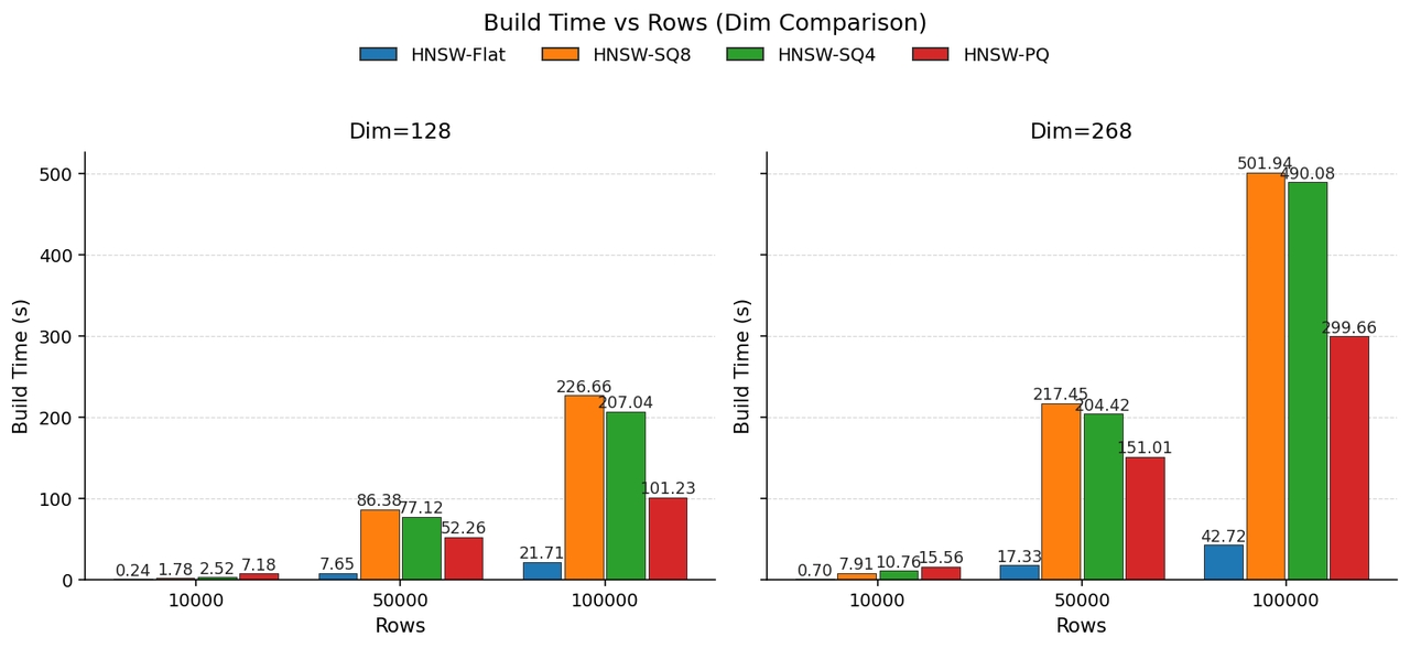
Vector Quantization

With FLAT encoding, an HNSW index (original vectors plus the graph structure) can consume a large amount of memory. HNSW must be fully resident in memory to work, so it easily becomes a bottleneck on very large datasets.

Doris provides two categories of quantization schemes:

Quantization	Principle	Doris Support
Scalar Quantization (SQ)	Compresses each FLOAT32 dimension to reduce memory overhead	sq8 (INT8), sq4 (INT4)
Product Quantization (PQ)	Decomposes a high-dimensional vector and quantizes each sub-vector separately	pq

Scalar Quantization (SQ) Example

CREATE TABLE sift_1M (
  id int NOT NULL,
  embedding array<float>  NOT NULL  COMMENT "",
  INDEX ann_index (embedding) USING ANN PROPERTIES(
      "index_type"="hnsw",
      "metric_type"="l2_distance",
      "dim"="128",
      "quantizer"="sq8"    -- Use INT8 for quantization
  )
) ENGINE=OLAP
DUPLICATE KEY(id) COMMENT "OLAP"
DISTRIBUTED BY HASH(id) BUCKETS 1
PROPERTIES (
  "replication_num" = "1"
);

In tests on the 768-dimensional Cohere-MEDIUM-1M and Cohere-LARGE-10M datasets, SQ8 compresses the index size to about 1/3 of FLAT.

Quantization Comparison

Dataset	Vector Dimension	Storage / Index Scheme	Total Disk Usage	Data Part	Index Part	Notes
Cohere-MEDIUM-1M	768D	Doris (FLAT)	5.647 GB (2.533 + 3.114)	2.533 GB	3.114 GB	1M vectors, raw + HNSW FLAT index
Cohere-MEDIUM-1M	768D	Doris SQ INT8	3.501 GB (2.533 + 0.992)	2.533 GB	0.992 GB	INT8 symmetric quantization
Cohere-MEDIUM-1M	768D	Doris PQ (pq_m=384, pq_nbits=8)	3.149 GB (2.535 + 0.614)	2.535 GB	0.614 GB	Product quantization
Cohere-LARGE-10M	768D	Doris (FLAT)	56.472 GB (25.328 + 31.145)	25.328 GB	31.145 GB	10M vectors
Cohere-LARGE-10M	768D	Doris SQ INT8	35.016 GB (25.329 + 9.687)	25.329 GB	9.687 GB	INT8 quantization, index significantly smaller

Product Quantization (PQ)

Doris also supports product quantization, but using PQ requires extra parameters:

• pq_m: The number of sub-vectors the original high-dimensional vector is split into. The vector dimension dim must be divisible by pq_m.
• pq_nbits: The number of bits used to quantize each sub-vector, which determines the codebook size of the subspace. In Faiss this is generally required to be no greater than 24.

Note

PQ quantization has training-data requirements during the training phase: at least as many points as there are cluster centers. That is, the number of training points n >= 2 ^ pq_nbits.

CREATE TABLE sift_1M (
  id int NOT NULL,
  embedding array<float>  NOT NULL  COMMENT "",
  INDEX ann_index (embedding) USING ANN PROPERTIES(
      "index_type"="hnsw",
      "metric_type"="l2_distance",
      "dim"="128",
      "quantizer"="pq",    -- Use PQ for quantization
      "pq_m"="2",          -- Required when using PQ. Number of low-dim sub-vectors the high-dim vector is split into
      "pq_nbits"="2"       -- Required when using PQ. Number of bits per subspace codebook
  )
) ENGINE=OLAP
DUPLICATE KEY(id) COMMENT "OLAP"
DISTRIBUTED BY HASH(id) BUCKETS 1
PROPERTIES (
  "replication_num" = "1"
);

Cost of Quantization

Quantization introduces extra build overhead: the build phase requires many distance computations, and each computation must decode the quantized values. For 128-dimensional vectors, build time grows with the row count, and SQ may introduce roughly 10x build cost compared to FLAT.

---

Performance Tuning

Vector search is a typical secondary-index point-query scenario. If you have high QPS and latency requirements, refer to the suggestions below. After tuning, on FE 32C 64GB + BE 32C 64GB machines, Doris can reach 3000+ QPS (dataset: Cohere-MEDIUM-1M).

Query Performance Benchmarks

Concurrency	Scheme	QPS	Avg Latency (s)	P99 Latency (s)	CPU Usage	Recall
240	Doris	3340.4399	0.071368168	0.163399825	40%	91.00%
240	Doris SQ INT8	3188.6359	0.074728852	0.160370195	40%	88.26%
240	Doris SQ INT4	2818.2291	0.084663868	0.174826815	43%	80.38%
240	Doris brute-force	3.6787	25.554878826	29.363227973	100%	100.00%
480	Doris	4155.7220	0.113387271	0.261086075	60%	91.00%
480	Doris SQ INT8	3833.1130	0.123040214	0.276912867	50%	88.26%
480	Doris SQ INT4	3431.0538	0.137636995	0.281631249	57%	80.38%
480	Doris brute-force	3.6787	25.554878826	29.363227973	100%	100.00%

Use Prepared Statements

Common embedding-model outputs are typically 768 dimensions or higher. If you embed such a vector as a literal directly in SQL, parsing time may exceed actual execution time. Therefore, prepared statements are recommended. Currently Doris does not support running these commands directly through the mysql client, so JDBC is required.

1. Enable server-side prepared statements in the JDBC URL.

   url = jdbc:mysql://127.0.0.1:9030/demo?useServerPrepStmts=true

2. Use the prepared statement.

   // use `?` for placement holders, readStatement should be reused
   PreparedStatement readStatement = conn.prepareStatement("SELECT id, l2_distance_approximate(embedding, cast (? as ARRAY<FLOAT>)) AS distance
       FROM l2_distance_approximate
       ORDER BY distance
       LIMIT 10");
     
   ...
   
   readStatement.setString("[0,11,77,24,3,0,0,0,28,70,125,8,0,0,0,0,44,35,50,45,9,0,0,0,4,0,4,56,18,0,3,9,16,17,59,10,10,8,57,57,100,105,125,41,1,0,6,92,8,14,73,125,29,7,0,5,0,0,8,124,66,6,3,1,63,5,0,1,49,32,17,35,125,21,0,3,2,12,6,109,21,0,0,35,74,125,14,23,0,0,6,50,25,70,64,7,59,18,7,16,22,5,0,1,125,23,1,0,7,30,14,32,4,0,2,2,59,125,19,4,0,0,2,1,6,53,33,2]");
   
   ResultSet resultSet = readStatement.executeQuery();

Reduce the Number of Segments

The Doris ANN index is built on segments. Too many segments introduce extra overhead.

• Recommendation: For tables with an ANN index, the number of segments per tablet should not exceed 5.
• How: Adjust write_buffer_size and vertical_compaction_max_segment_size in be.conf to enlarge a single segment and reduce the count. Setting both to 10737418240 (10 GB) is recommended.

Reduce the Number of Rowsets

Each load creates one rowset, and too many rowsets also increase scheduling overhead. Use Stream Load or INSERT INTO SELECT for batch loading.

Keep ANN Indexes Resident in Memory

The current ANN index algorithm is memory-based. If a queried segment's index is not resident in memory, it triggers disk I/O. For performance, keep it resident by setting in be.conf:

enable_segment_cache_prune=false

parallel_pipeline_task_num = 1

ANN TopN queries return very few rows and do not need high parallelism. Use:

SET parallel_pipeline_task_num = 1;

enable_profile = false

If latency is extremely sensitive, disable the query profile:

SET enable_profile = false;

---

Python SDK

In the AI era, Python has become the mainstream language for data processing and intelligent application development. To make it easier for developers to use Doris vector search in Python, the community contributed a Python SDK:

• doris_vector_search: Optimized for vector distance retrieval. Currently the best-performing Doris vector-search Python SDK.

---

Usage Limitations

When using the Doris vector index, note the following limitations:

1. Data type limitation: The column on which an ANN Index is built must be a NOT NULLABLE Array<Float>. During data load, the length of every vector in this column must equal the dimension specified in the index property (dim), otherwise an error is reported.

2. Table model limitation: ANN Index can only be used on the Duplicate Key table model.

3. Predicate columns must have a secondary index: Doris uses pre-filter semantics (predicates are evaluated before AnnTopN). When the columns referenced by predicates in the SQL do not have a secondary index, Doris falls back to brute-force computation to ensure correctness. For example:

   SELECT id, l2_distance_approximate(embedding, [xxx]) AS distance
       FROM sift_1M
       WHERE round(id) > 100
       ORDER BY distance limit 10;

   Although id is the primary key, no secondary index (such as inverted) that can precisely locate row numbers has been built on this column. Such predicates are evaluated after index analysis. To preserve the pre-filter semantics of ANN TopN, the system falls back to brute-force computation.

4. The distance function must match the metric type: If the distance function used in the SQL does not match the metric_type of the index defined in the DDL, Doris cannot use the ANN index for TopN computation (even when you use l2_distance_approximate / inner_product_approximate).

5. inner_product must use DESC sorting: When metric_type is inner_product, only ORDER BY inner_product_approximate() DESC LIMIT N (DESC cannot be omitted) can be accelerated by the ANN index.

6. Function argument order: The xxx_approximate() function triggers index analysis only when the first argument is a ColumnArray and the second argument is a CAST or ArrayLiteral. Swapping the order causes a fallback to brute-force search.

---

FAQ

Q1: Which distance metrics does the Doris ANN index support?

Currently l2_distance (Euclidean distance) and inner_product are supported. For cosine similarity, see the Using Cosine Similarity section.

Q2: Why does my ANN query not use the index?

Possible reasons:

• The distance function does not match the metric_type.
• When using inner_product, ORDER BY ... DESC was not used.
• Function argument order is reversed (ColumnArray must be the first argument).
• The filter columns lack a secondary index such as an inverted index, triggering a brute-force fallback.

Q3: How do I choose between HNSW, IVF, and IVF On-Disk?

Index	Memory Usage	Query Performance	Applicable Scenarios
HNSW	High (must be fully resident in memory)	High	Small-to-medium scale, strong low-latency requirements
IVF	Medium	Medium	Large-scale data
IVF On-Disk	Low (on-disk + cache)	Medium	Very large-scale data, memory-constrained

Q4: What if I do not have enough memory?

Reduce memory usage through quantization:

• Try sq8 (INT8 scalar quantization) first. It typically compresses the index to about 1/3 of the original size with limited recall impact.
• When memory is very tight, use sq4 or pq, but recall will drop somewhat.

Q5: How do I combine keyword filtering with vector retrieval?

Build an inverted index on the filter columns, then use an ANN query with a WHERE clause. See ANN Search with Filters.

Q6: How do I improve QPS?

See the Performance Tuning section. Key points:

• Use prepared statements to avoid SQL parsing overhead.
• Reduce the number of segments and rowsets.
• Keep the ANN index resident in memory.
• parallel_pipeline_task_num = 1.
• Disable the query profile.