Product Concepts
This document introduces the core product concepts of Apache Doris and serves as the foundation for understanding other documentation. These concepts cover key dimensions such as data organization, storage models, query execution, and query optimization.
Applicable scenarios: Concept introduction, reading preparation, technical warm-up
Data Organization
Catalog / Database / Table
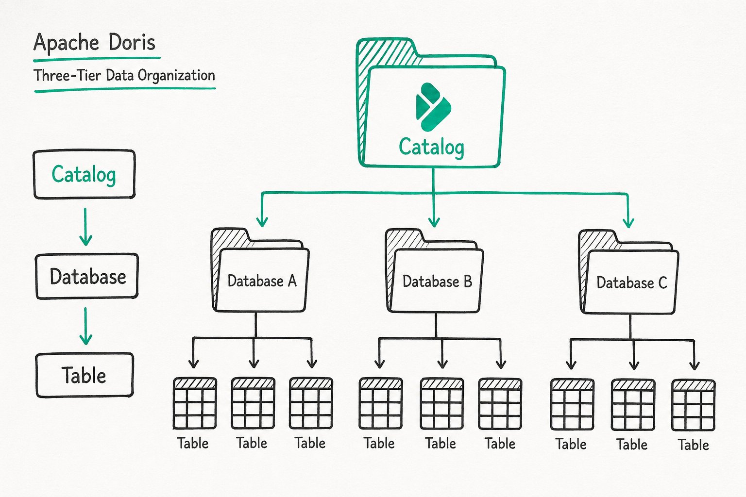
Apache Doris adopts a three-tier hierarchy of Catalog → Database → Table to manage data.
| Tier | Description |
|---|---|
| Catalog | A logical namespace used to distinguish different data sources. The default internal Catalog in Doris represents internal storage, holding the Databases and Tables created by users. External Catalogs can connect to data sources such as Hive, Iceberg, and MySQL, enabling cross-source queries without data migration. |
| Database | A database unit used to isolate data belonging to different businesses or projects. You can configure attributes such as character set and collation. |
| Table | A two-dimensional relational table that defines the column structure (Schema) and table properties (bucketing rules, lifecycle, and so on). It is the basic unit of data storage and querying. All queryable objects in Doris are presented in the form of a Table. |
Why a three-tier design?
The tiered design balances logical isolation with unified cross-source access. Business teams own independent Databases, while platform teams can directly query data from other data sources through External Catalogs.
Internal Catalog
The Internal Catalog is the default built-in Catalog of Doris. Its name is fixed as internal, and it manages tables and data stored in the Doris internal format.
Responsibilities:
- Stores all user-created Databases (
CREATE DATABASE) - Stores all user-created Tables (
CREATE TABLE) - Manages the import, compression, and version merging (Compaction) of internal data
When a user runs SHOW DATABASES or USE my_db, the operation runs in the Internal Catalog context by default.
External Catalog
An External Catalog is a logical component that connects to external data sources, allowing direct queries against external data without data migration.
| External Data Source | Description |
|---|---|
| Hive | Connects to Hive Metastore or HMS-compatible data lakes |
| Iceberg | Connects to Iceberg tables |
| Paimon | Connects to Paimon tables |
| JDBC | Connects to relational databases such as MySQL, PostgreSQL, and OceanBase |
Special note for Iceberg and Paimon:
These two data sources support full data management capabilities, including DDL operations (CREATE/DROP/ALTER TABLE) and DML operations (INSERT/UPDATE/DELETE), not only queries. You can manage Iceberg/Paimon table schemas directly in Doris and perform data writes.
Use cases:
- Data lake analytics: Analyze Hive/Iceberg/Paimon data directly without ETL
- Cross-source queries: Query an Iceberg data source and Doris data within a single SQL statement
How to use: After creating an External Catalog, you can query it directly with SELECT * FROM catalog.database.table. You can also switch to the corresponding Catalog with SWITCH catalog.
Internal Catalog vs. External Catalog
| Comparison | Internal Catalog | External Catalog |
|---|---|---|
| Name | Fixed as internal | User-defined |
| Data format | Doris internal format (columnar storage) | External data source format (Parquet, ORC, etc.) |
| Data storage location | BE node local disks or object storage | External systems (HDFS, S3, Hive Metastore, etc.) |
| Creation method | CREATE DATABASE / CREATE TABLE | CREATE EXTERNAL CATALOG |
| Query performance | High (data is local) | Depends on the external data source. Doris also provides multiple built-in acceleration mechanisms |
| DDL/DML support | Fully supported | Iceberg/Paimon fully supported; Hive/JDBC supports queries only |
| Data writes | Supported (Stream Load, etc.) | Only Iceberg/Paimon are supported |
Partition and Bucket
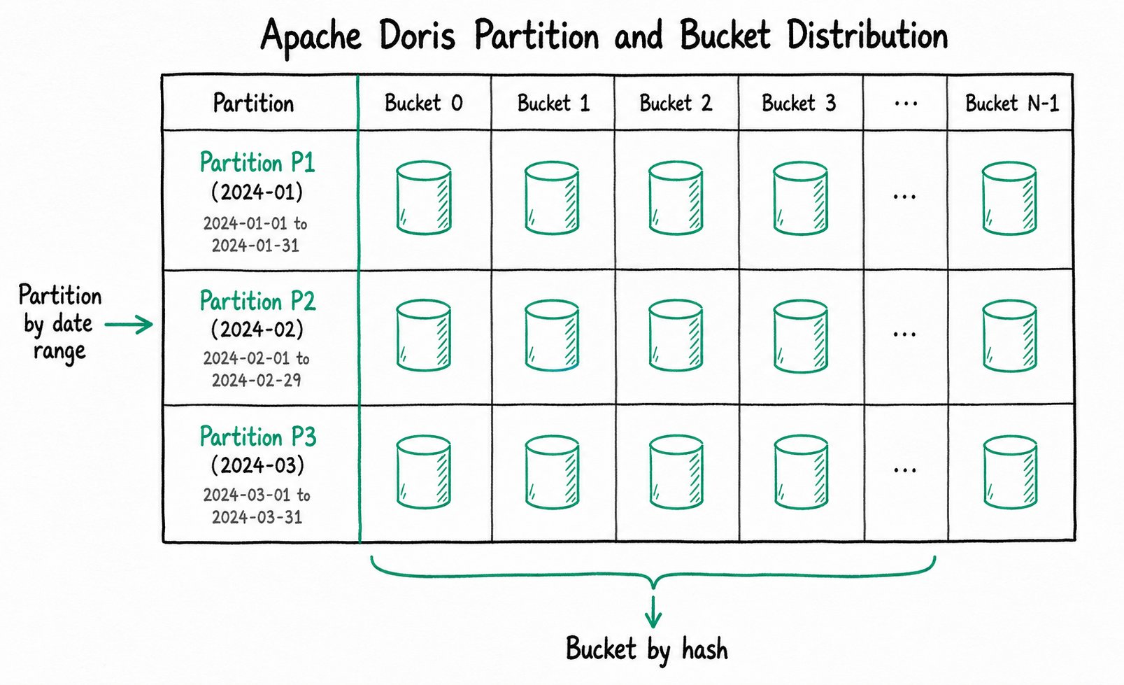
A partition horizontally splits the data in a table by the value range of a specific column. A table can contain one or more partitions, and each partition corresponds to a continuous data range.
Typical uses:
- Time-based partitioning (by day/month/year), which supports partition pruning and historical data management
- Region-based or business-line partitioning for data isolation
Example: A log table is partitioned by day on the date column.
Partition p20240101: data where date = '2024-01-01'
Partition p20240102: data where date = '2024-01-02'
Partition p20240103: data where date = '2024-01-03'
When you run WHERE date = '2024-01-02', Doris scans only the p20240102 partition and skips the others, greatly reducing I/O.
A bucket horizontally splits the data in a table based on the hash value of a specific column or the number of buckets, and determines the physical distribution of data across the cluster.
The physical storage that corresponds to a bucket is called a Tablet, which is the smallest logical unit of storage.
| Concept | Description |
|---|---|
| Distribution Key | The column used to compute which bucket a row belongs to. Choose a high-cardinality column such as a primary key ID. |
| Bucket Num | The number of physical buckets in a partition. It determines the parallelism of the data. |
Differences between buckets and partitions:
| Dimension | Partition | Bucket |
|---|---|---|
| Division basis | Value range of a column | Hash computation |
| Purpose | Data lifecycle management, partition pruning | Parallel data distribution, JOIN optimization |
| Hierarchy | A partition contains buckets | A bucket belongs to a partition |
A partition defines the logical boundary of data (such as a time range), and a bucket defines the physical distribution of data (such as how data is spread across cluster nodes).
Storage Model
Columnar Storage
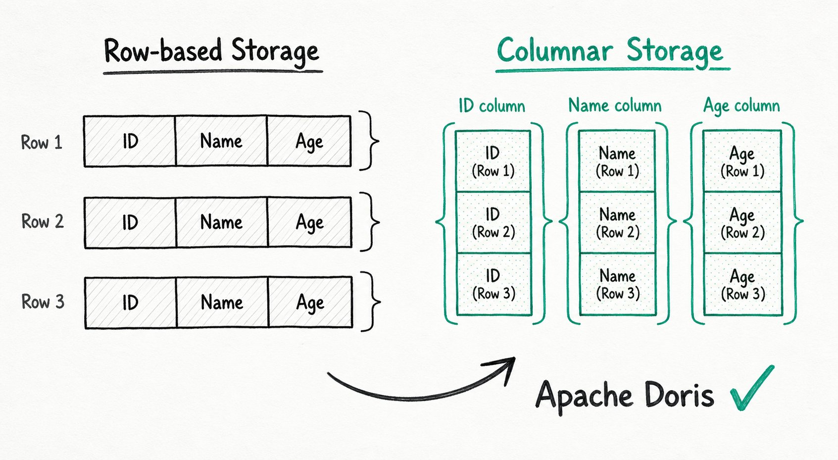
Columnar storage is a format that organizes data by column rather than by row.
Row-based storage vs. columnar storage:
Row-based storage (each row is stored contiguously):
[row1: id=1, name=alice, age=30] [row2: id=2, name=bob, age=25] ...

Columnar storage (each column is stored contiguously):
[id column: 1, 2, 3, ...] [name column: alice, bob, carol, ...] [age column: 30, 25, 28, ...]
Advantages of columnar storage:
| Advantage | Description |
|---|---|
| High I/O efficiency | A query reads only the columns it needs, avoiding a full table scan. For report queries that touch only a few columns, I/O can drop by tens of times. |
| High compression ratio | Data within the same column shares one type, which is well suited to algorithms such as dictionary encoding, bitmap compression, and RLE, significantly reducing storage space. |
| Vectorization-friendly | Data within the same column is stored contiguously in memory, leading to high CPU cache hit rates and enabling high-speed computation with SIMD instructions. |
Data Models
Doris supports three data models that handle different data merging requirements across business scenarios.
| Model | Description | Use Cases |
|---|---|---|
| Duplicate | Retains all original data; multiple records with the same key are all preserved. | Detail storage of fact tables, log analytics |
| Aggregate | Records with the same key are merged according to aggregation functions (such as SUM, MAX, MIN). | Metric statistics, report pre-aggregation |
| Primary Key | Keys are unique; records with the same key overwrite previous ones (supports row-level updates). | Real-time updates, CDC data ingestion |
Example:
Suppose you have the following raw data (the primary key is user_id):
| user_id | visit_date | pv |
|---|---|---|
| 1 | 2024-01-01 | 5 |
| 1 | 2024-01-01 | 3 |
| 2 | 2024-01-01 | 10 |
- Duplicate model: All 3 records are retained.
- Aggregate model (with SUM aggregation):
pvvalues for the same key are merged, so user_id=1 has pv=8 and user_id=2 has pv=10. - Primary Key model: Records with the same key are overwritten by timestamp, leaving only the latest one (for example,
pv=3overwritespv=5).
Query Execution
MPP (Massively Parallel Processing)
MPP is a massively parallel processing architecture used to execute complex queries.
Core concepts:
| Concept | Description |
|---|---|
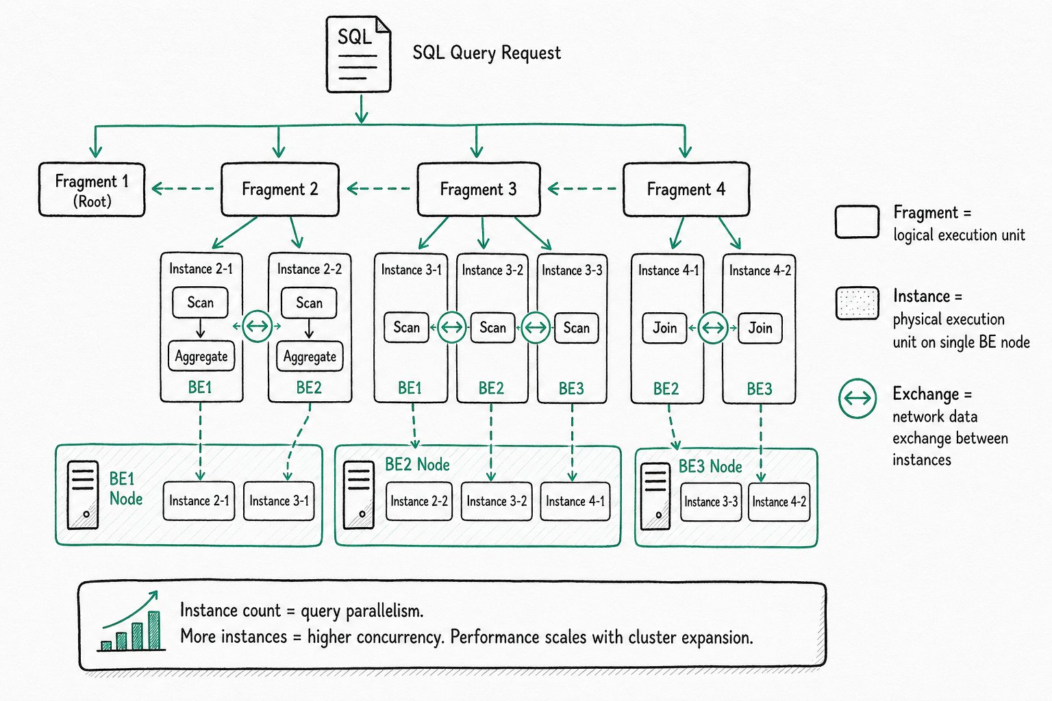
| Fragment | A logical execution unit. A query plan consists of multiple Fragments. |
| Instance | A physical execution unit composed of a group of operators (such as Scan, Agg, Join) that can run on a single BE node. |
| Exchange | The operator that performs network data exchange between Instances. |
How it works:
- The FE parses the SQL and generates a logical execution plan.
- The plan is split into multiple Fragments (logical execution units).
- Each Fragment is instantiated as one or more Instances and dispatched to multiple BE nodes for parallel execution.
- Different Instances exchange data over the network through the Exchange operator.
- After each node finishes execution, the results are aggregated at the FE.
Instance and parallelism:
An Instance is the physical execution unit of a query, runs on a single BE node, and contains a group of operators (Scan → Agg → Join, and so on). The number of Instances equals the parallelism of the query: more Instances means higher concurrency. Each execution node owns dedicated resources (CPU and memory), and a single query request can fully utilize the resources of all execution nodes. As a result, query performance scales as the cluster scales out horizontally.
Use cases: Operations that require cross-node data exchange, such as large-table JOINs, GROUP BY, and ORDER BY.
Vectorized Execution Engine
Vectorized execution is an execution method that processes data in column-wise batches and uses SIMD instructions to accelerate computation.
Traditional row-based execution vs. vectorized execution:
| Dimension | Row-based execution | Vectorized execution |
|---|---|---|
| Processing unit | One row at a time | One column (a batch) at a time |
| CPU cache | Random access, low cache hit rate | Sequential access, high cache hit rate |
| SIMD instructions | Hard to leverage | Fully utilized |
| Aggregation performance | Baseline | 5-10x improvement |
Core idea: Change the inner loop of an operator from "process one row" to "process one column (a batch of data)" to reduce function call overhead and improve CPU utilization.
Pipeline Execution Engine
Pipeline is a multi-core parallel execution model that maximizes the use of multi-core resources through pipelined parallelism.
Problems it solves:
- Thread explosion: Traditional models allocate a fixed number of threads per query, causing the thread count to spiral out of control as queries surge.
- Resource contention: A fixed-size thread pool causes resource contention between queries.
Pipeline characteristics:
| Feature | Description |
|---|---|
| Thread count limit | Parallelism is limited by the number of CPU cores, not by the number of queries. |
| Operator-chain scheduling | Upstream and downstream operators form a pipeline, and data flows through continuously. |
| Reduced blocking | Reduces thread switching and lock contention, improving throughput. |
Within a single query, multiple operators form a parallel pipeline. At the cluster level, multiple queries share CPU resources, enabling efficient multi-tenant scheduling.
Query Optimization
Materialized View
A materialized view is a precomputation technique that stores query results as a physical table and updates them automatically as data is loaded.
Core value:
| Feature | Description |
|---|---|
| Query rewrite | When a user queries the original table, the optimizer automatically determines whether the query can be transparently rewritten to read from the materialized view. The user does not need to change the SQL. |
| Automatic synchronization | The materialized view is updated automatically as the source table changes, with no manual maintenance required. |
| ETL replacement | It can replace traditional scheduled ETL pipelines and provide real-time acceleration. |
Use cases:
- Aggregation queries on large tables (such as report rollups)
- Layered modeling in data warehouses (fact tables → summary tables)
- Precomputing complex JOIN results
CBO (Cost-Based Optimizer)
The CBO is a cost-based query optimizer. It estimates the resource consumption (I/O, CPU, network) of each candidate execution plan and selects the lowest-cost plan.
Typical scenarios optimized by the CBO:
| Optimization | Description |
|---|---|
| Join order | For multi-table JOINs, the CBO evaluates the cost of different orders and picks the best one. |
| Join algorithm | The CBO picks Hash Join, Nest Loop Join, or Broadcast Join based on data volume. |
| Distributed execution | The CBO decides which nodes execute and whether a Shuffle is needed. |
Why is the CBO needed? SQL describes only "what to do," not "how to do it." For the same query, the optimal execution path can differ entirely depending on data volume. The CBO uses statistics (row count, column cardinality, NDV, and so on) to estimate cost and choose the most efficient execution path.
RBO (Rule-Based Optimizer)
The RBO is a rule-based optimizer. It rewrites the logical plan according to predefined rules, without considering actual data characteristics.
Typical optimization rules:
| Rule | Description |
|---|---|
| Constant folding | 1 + 2 → 3 |
| Predicate pushdown | Filter conditions run before the JOIN to reduce intermediate results. |
| Subquery rewriting | Flatten nested subqueries into JOINs. |
| Common expression reuse | An expression that appears multiple times is computed only once. |
CBO vs. RBO: The RBO is deterministic and rule-driven, which fits scenarios with fixed rules. The CBO is smarter and can optimize based on data characteristics, but it relies on accurate statistics. Doris uses both: the RBO handles deterministic optimizations, and the CBO handles complex plan selection.
Runtime Filter
A Runtime Filter is a filter condition generated dynamically during query execution and pushed down to the scan node, so that filtering happens during the data read phase.
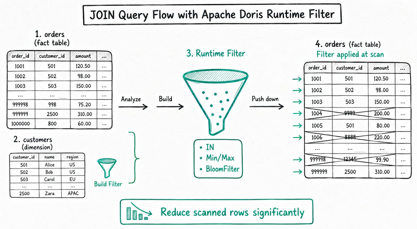
How it works:
Suppose a JOIN is performed between the large table orders and the small table customers on customer_id:

1. The FE analyzes the small table and builds a Filter (such as customer_id IN {1, 5, 9}).
2. The Filter is pushed down to the nodes that scan the large table.
3. While the large table is being read, rows that do not match are filtered out immediately and skipped.
4. This reduces I/O and the workload of subsequent operators.
Runtime Filter types:
| Type | Use Cases |
|---|---|
| IN | Small table joins large table, equi-JOIN |
| Min/Max | Range JOIN, continuous data distribution |
| BloomFilter | High-cardinality column, equi-JOIN |
Effect: In a star schema, when a large fact table joins a small dimension table, a Runtime Filter can reduce the scan volume of the large table by several to tens of times.
FAQ
Q: What is the difference between partitions and buckets?
A partition divides data by the value range of a column. It is used for data lifecycle management (such as deleting historical data by daily partitions) and partition pruning (scanning only the relevant partitions for a query). A bucket distributes data by hash for parallel processing and JOIN optimization. A partition is a logical concept; a bucket is a physical concept (it determines which BE node a piece of data is distributed to).
Q: When should I choose the Primary Key model instead of the Duplicate model?
Choose the Primary Key model when you need row-level updates (such as real-time data ingestion or CDC synchronization), or when you want records with the same key to be merged. The Duplicate model retains all original data and fits log analytics and full-detail query scenarios.
Q: How are MPP and Pipeline related?
They are parallel mechanisms at two different dimensions. MPP is distributed parallelism, which addresses parallel computation across nodes. Pipeline is intra-node parallelism, which addresses utilization of multi-core resources. Together they deliver end-to-end parallelism: "parallelism between nodes plus pipelining within a node."
Q: Where do CBO and RBO statistics come from?
Doris collects table and column statistics with the ANALYZE command, including table row count, column cardinality (NDV), NULL ratio, and so on. The CBO relies on these statistics for cost estimation. More accurate statistics produce better optimization results. Run ANALYZE again after a significant change in data volume.
Q: What is the difference between an External Catalog and a regular Database?
A regular Database stores data inside Doris, while an External Catalog is only a logical mapping, with the actual data still stored in the external data source. Doris reads external data directly through the External Catalog, with no ETL migration required. Common use cases include querying data lakes (Hive/Iceberg/Hudi) and running cross-source queries (MySQL, PostgreSQL, and so on).
Q: What is the difference between a materialized view and a regular view?
A regular view only stores the SQL query logic and computes the result every time it is queried, providing no performance benefit. A materialized view physically stores the query result, keeps the data in sync, and transparently accelerates user queries. Materialized views fit aggregation report scenarios with stable patterns.
Further Reading
- [TODO] - Learn about the integrated and disaggregated storage-compute architectures
- [TODO] - Deep dive into the CBO and execution plans